Test E: Colliding
outflows -- 2D test of 3D code
- Domain and execution:
- 33x33x16 grid - runs quickly for interactive testing
- (note odd dimension
for nx,ny; initial bubble at exact X-Y center)
- ∆x=∆y=∆z = 500
meters
- ∆t = 1.0 seconds; run to 450s
- Save data (via
putfield)
at 150, 250, 350 and 450s (and other times if you
wish).
- Physics:
- All processes
retained and active.
- Sound speed Cs=100 m/s.
- Non-monotonic
piecewise linear advection.
- Diffusion
coefficients = 50 (momentum), 5 (temperature).
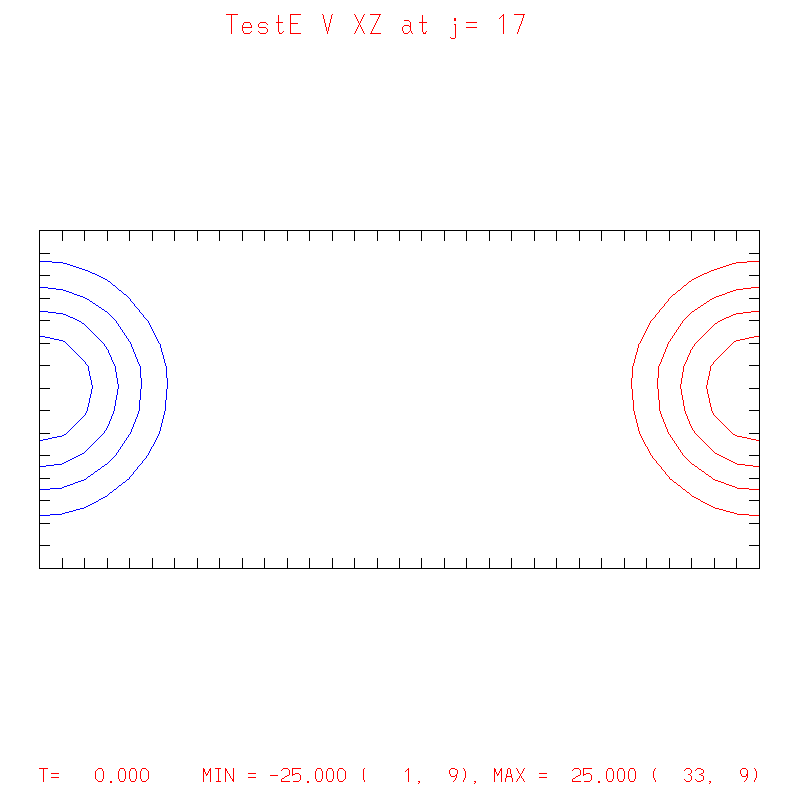
- Initial
condition:
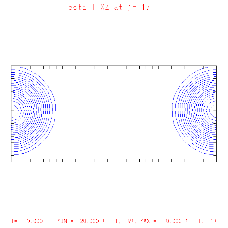
- Theta: 2 thermals:
- -20˚,
center ( 250,8250,4250)
- -20˚, center (16250,8250,4250)
- radius
= 4000m in each direction X and Z, 999999 meters
in Y to create ~2D initial condition
- U,W: are initially zero - no perturbations on U
- V (using same
formula as for theta) has -25 m/s max perturbation
for "left boundary thermal", and +25m/s on right.
- Boundary conditions:
- Usual (symmetric X, periodic Y, 0-gradient Z)
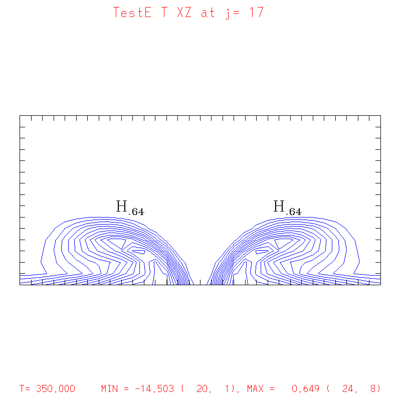
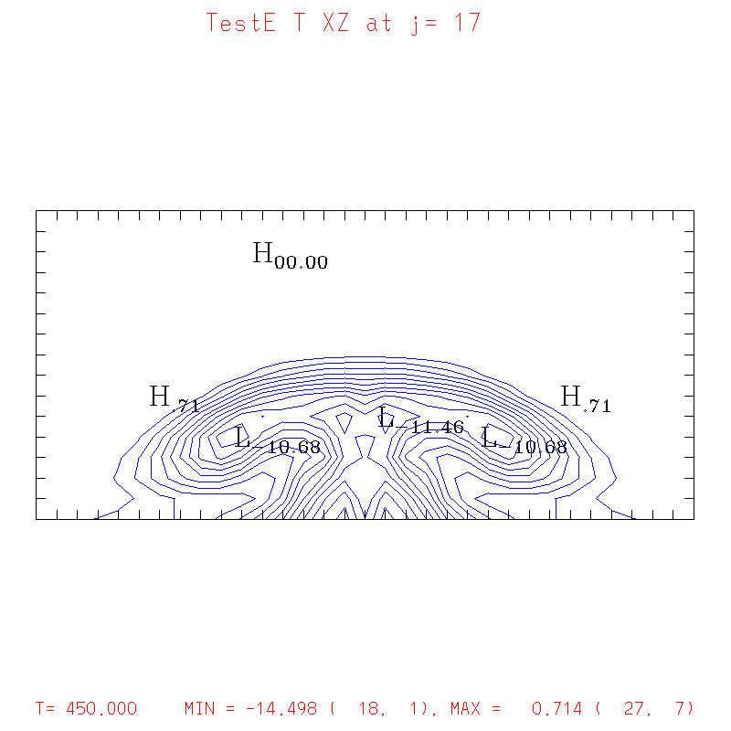
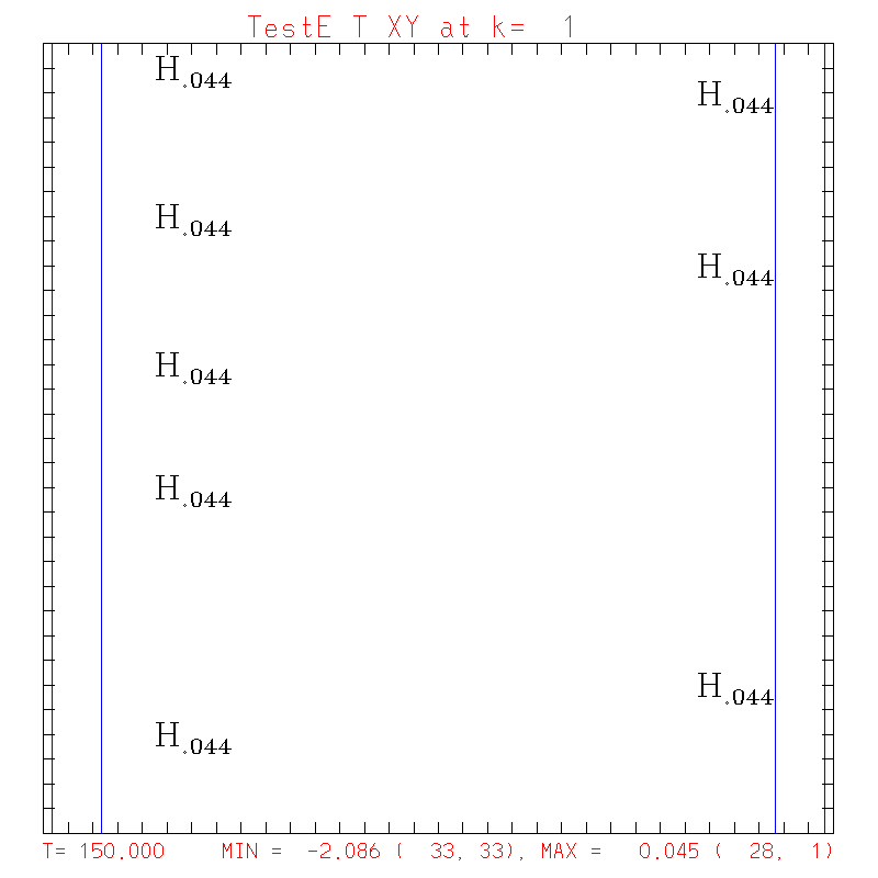
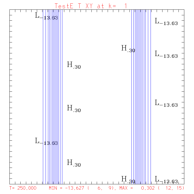
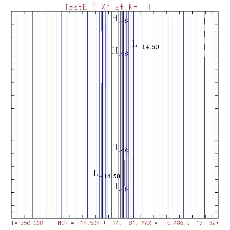
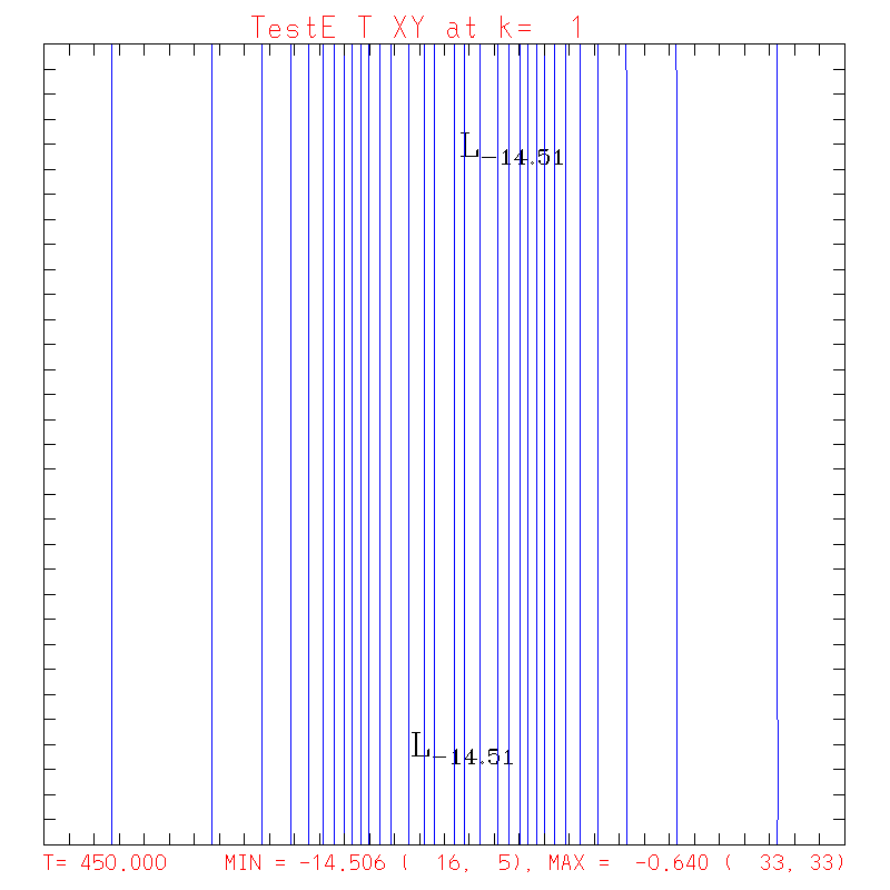
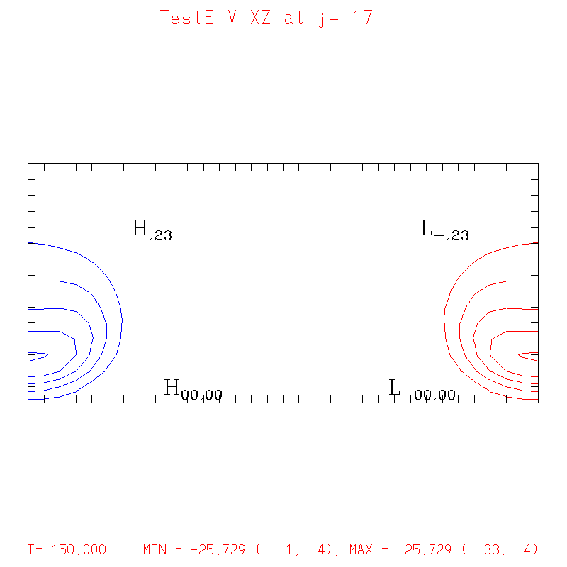
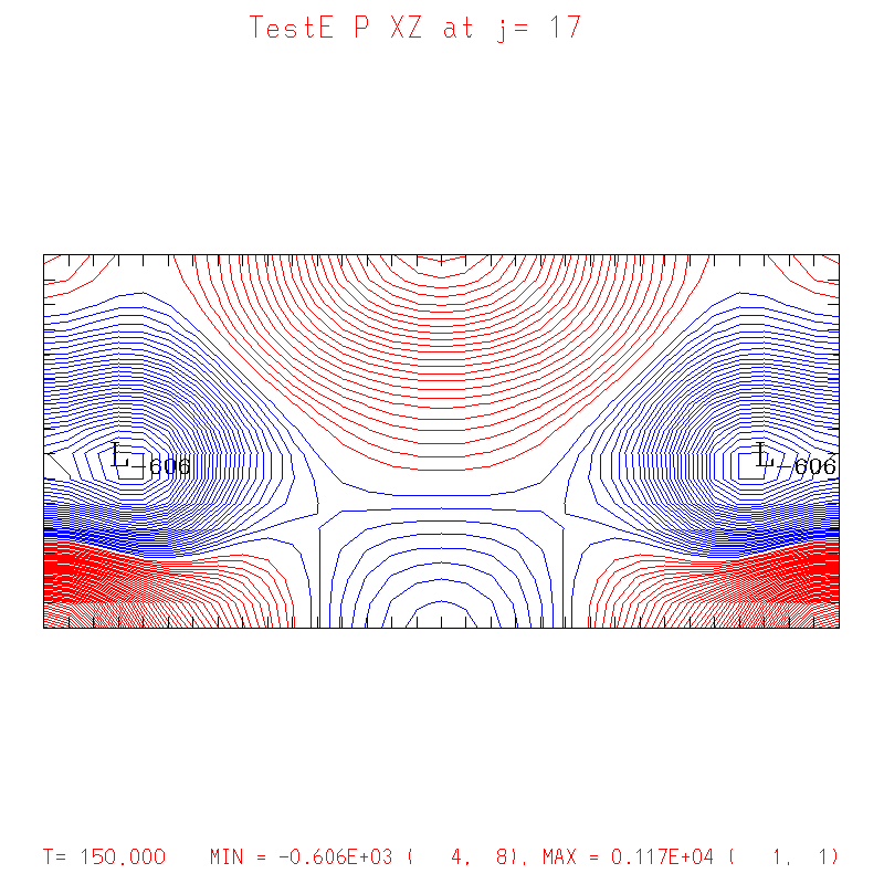
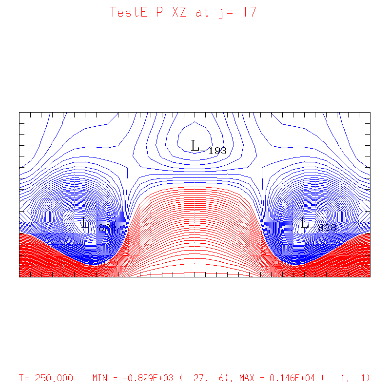
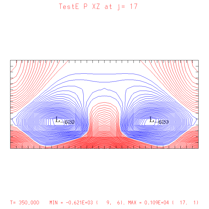
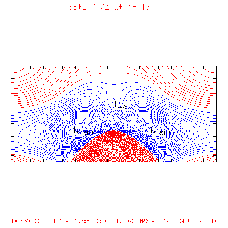
Test E: Colliding density currents
- This is a 2-D test of your 3-D code. Without U
perturbations, it is a 2D initial state, and the
solution should remain 2D. In particular, when
evaluating your solution you should look for any
evidence of along-line (i.e. in Y-direction) variation
to your fields, and you should also find no noise on
the periodic Y boundaries. I have omitted Y-Z
plots below for obvious reasons, but you can compute
them -- they should show only height variation (in
plotted Y-Z slices).
- Text output from running my code may be found
here.
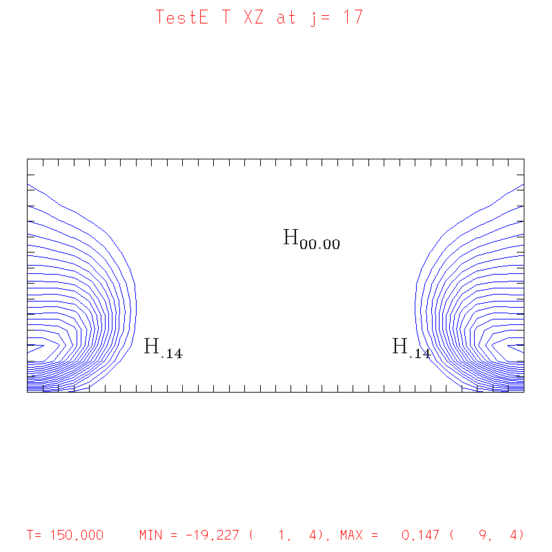
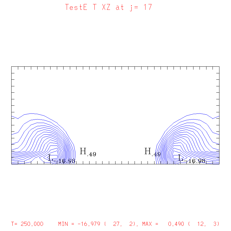
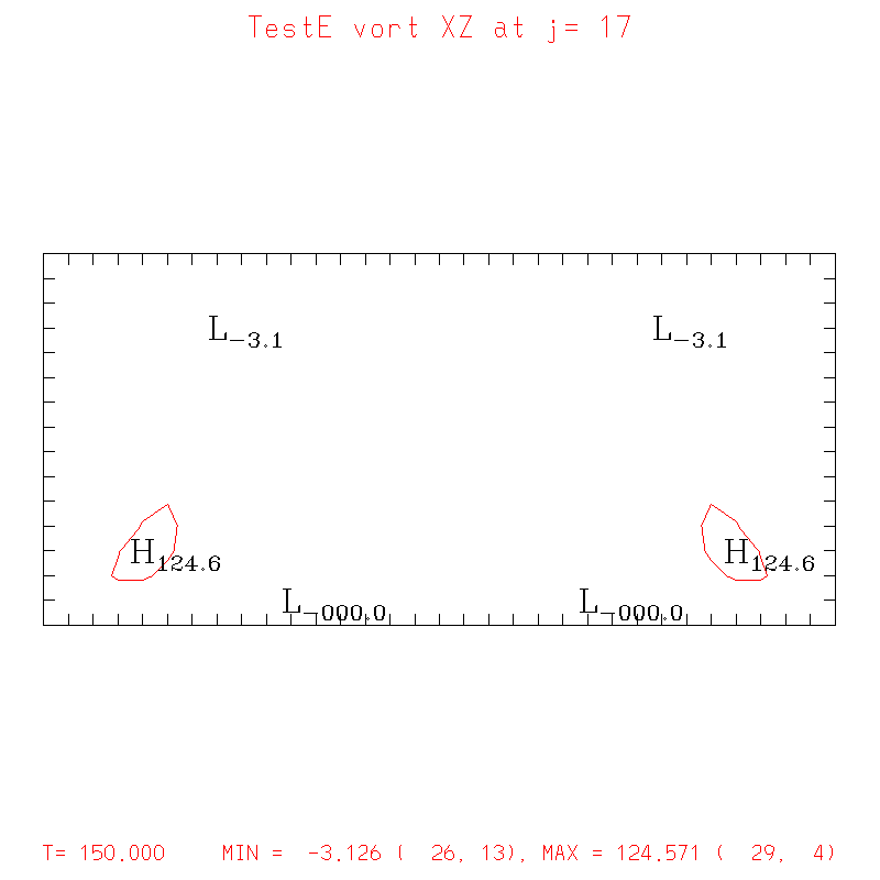
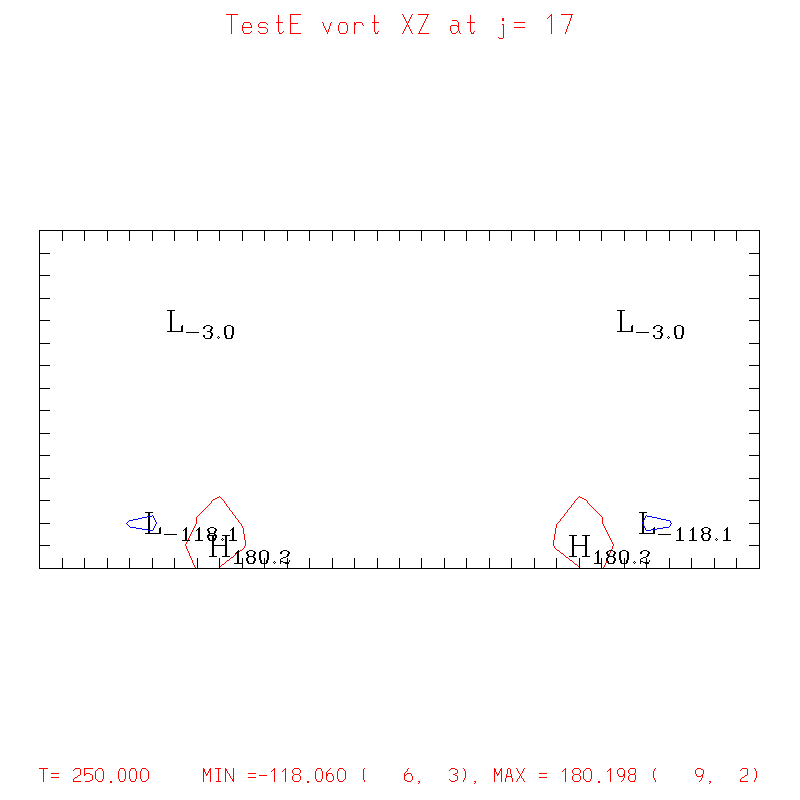
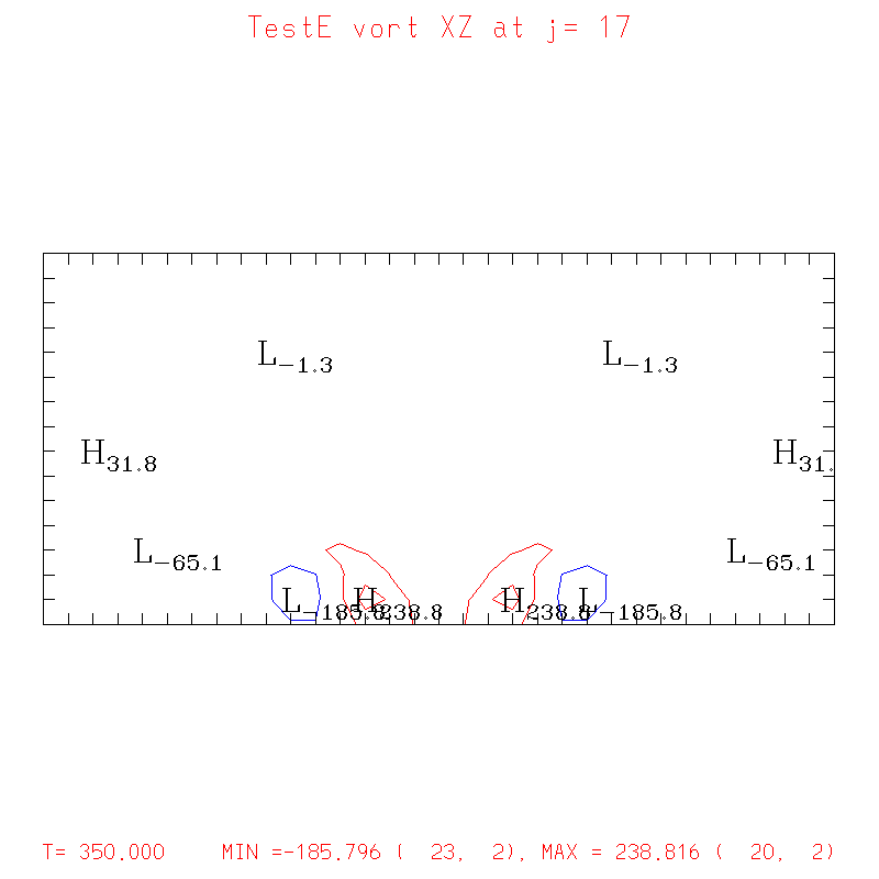
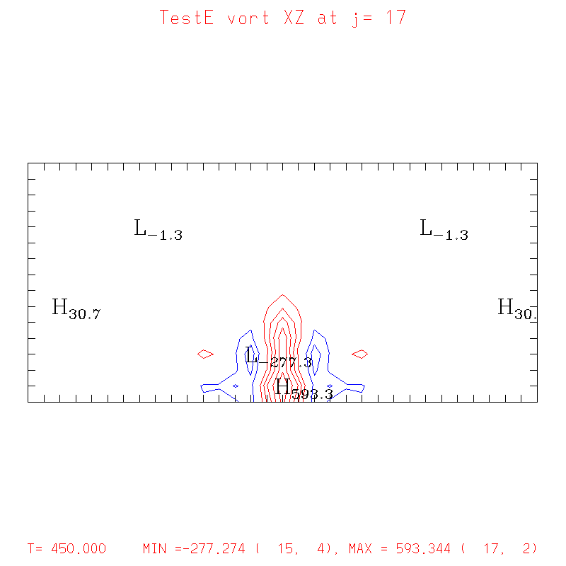
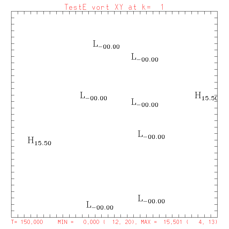
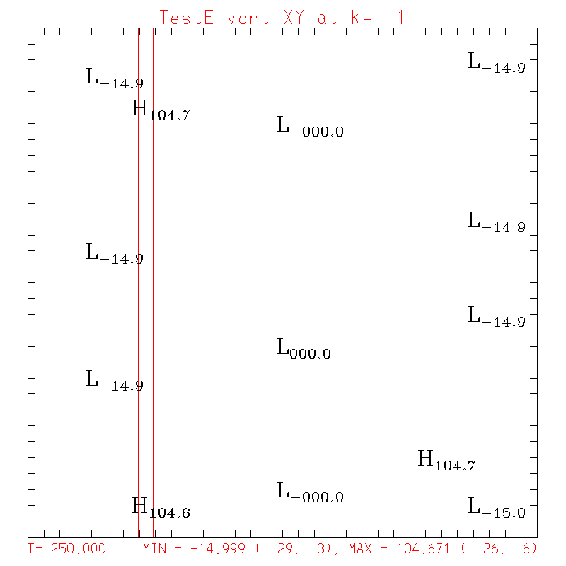
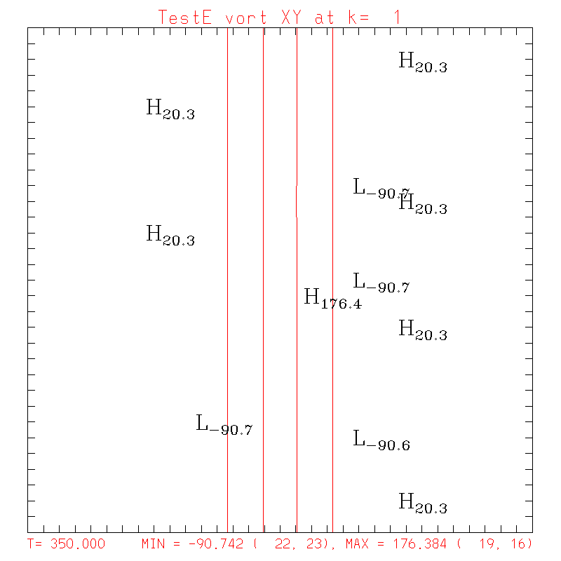
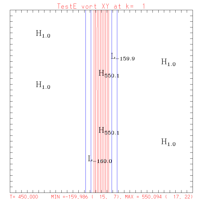
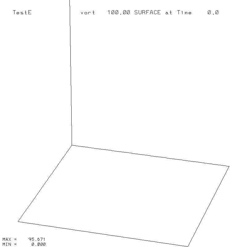
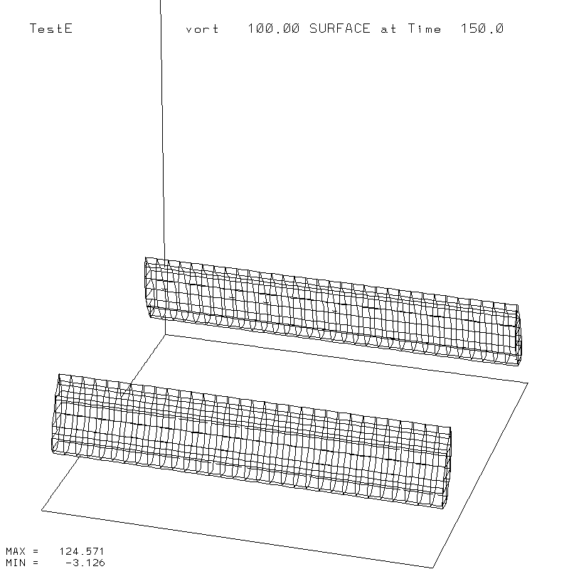
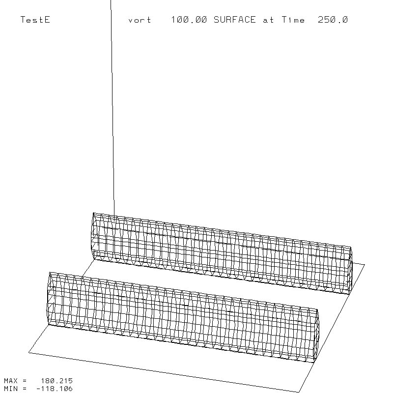
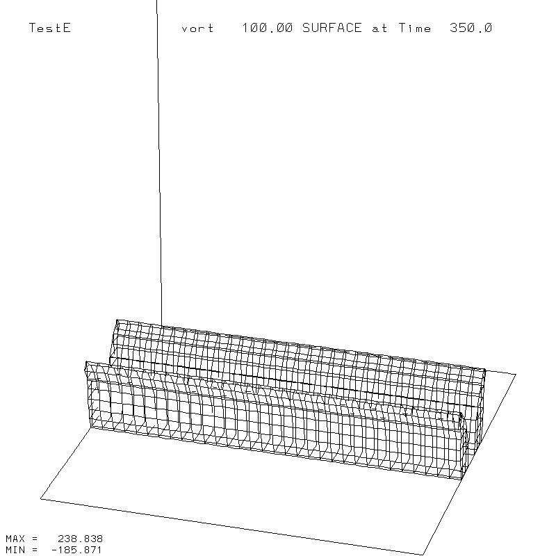
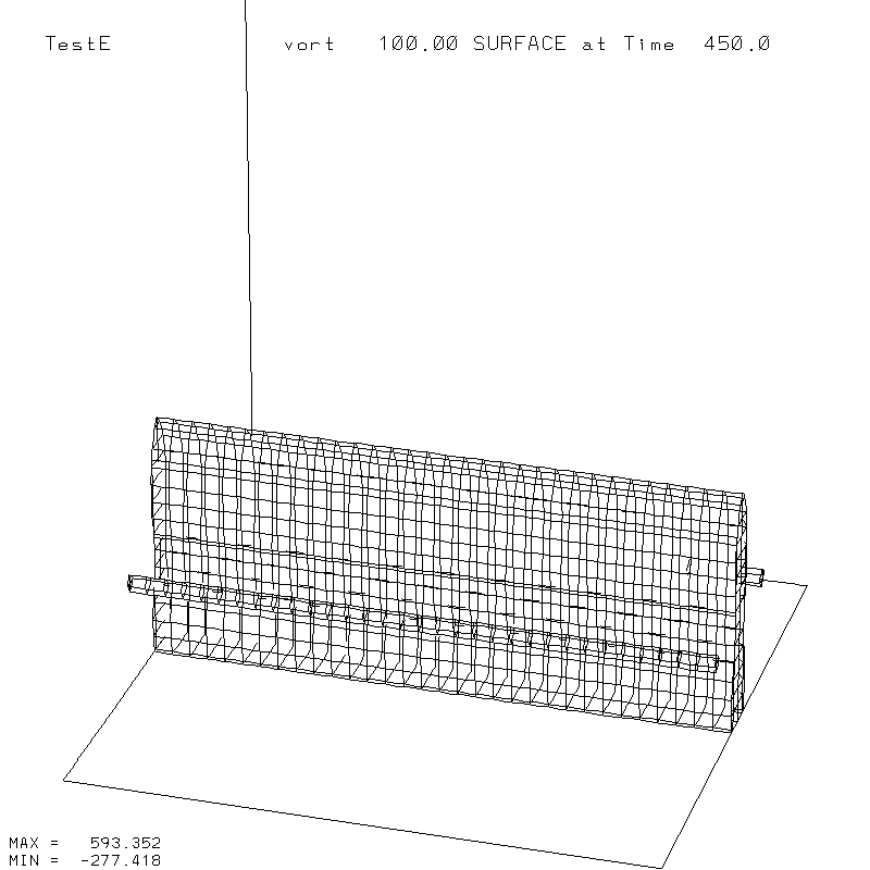
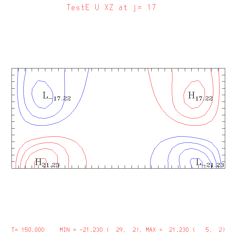
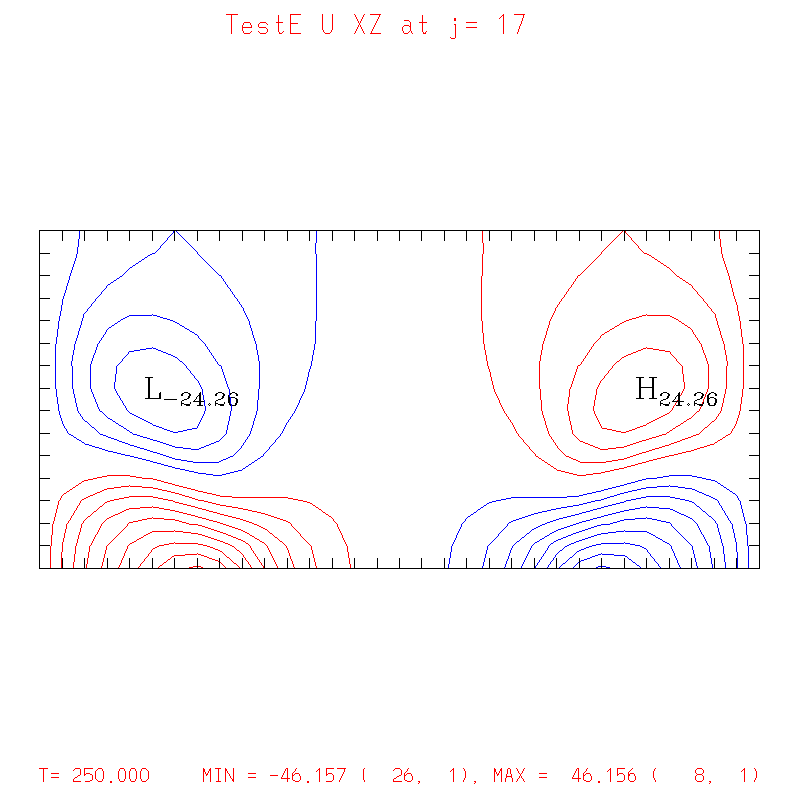
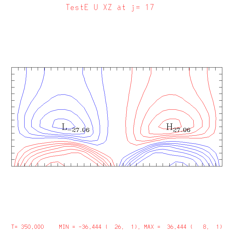
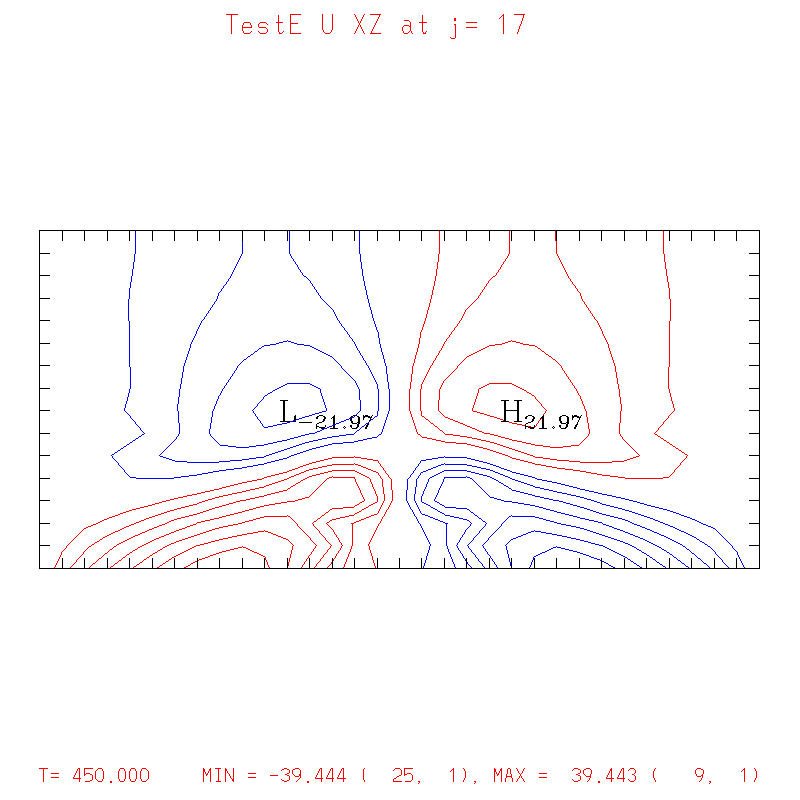
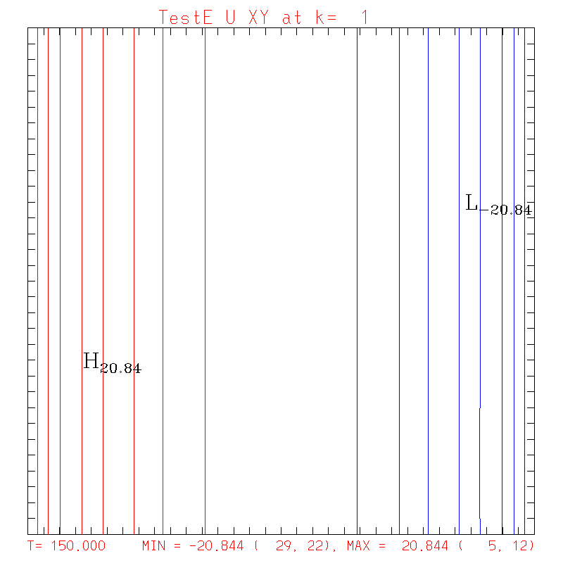
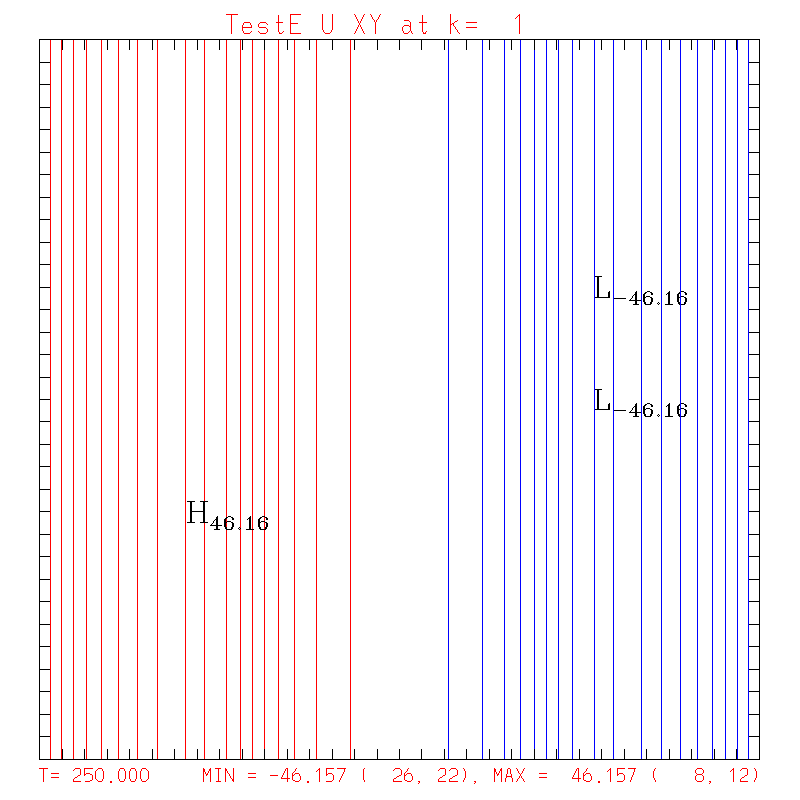
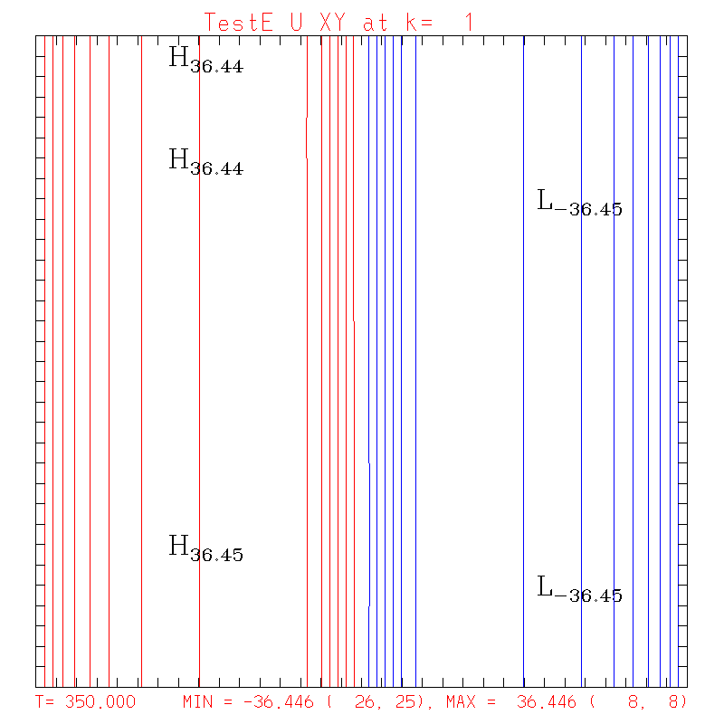
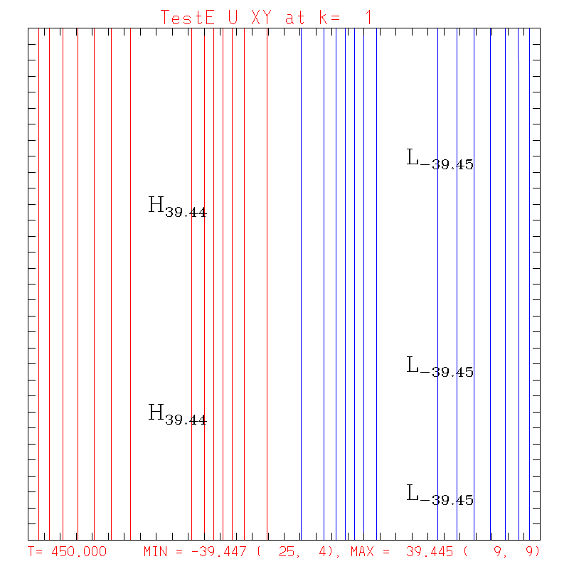
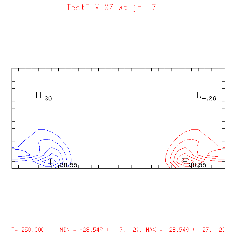
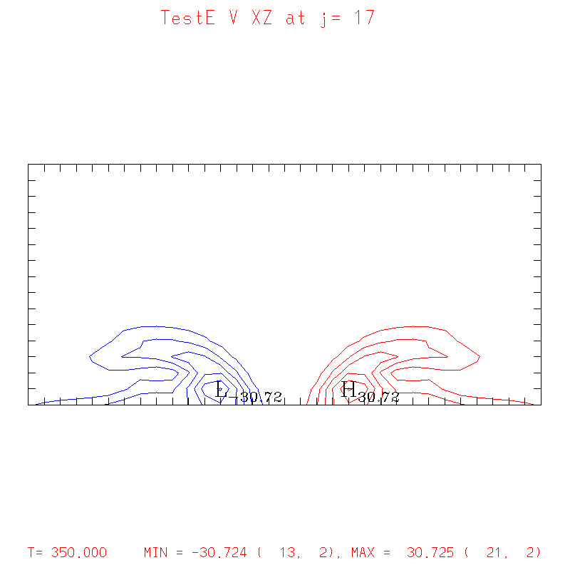
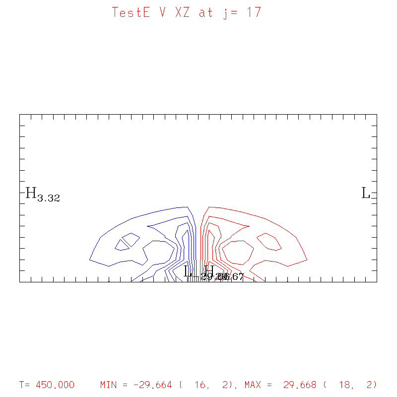
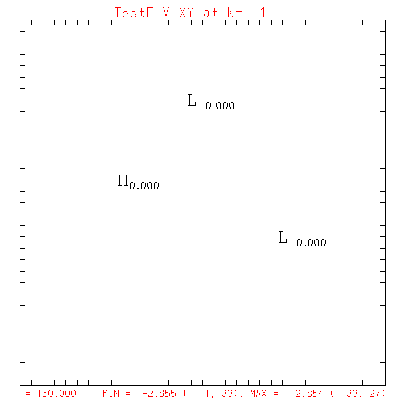
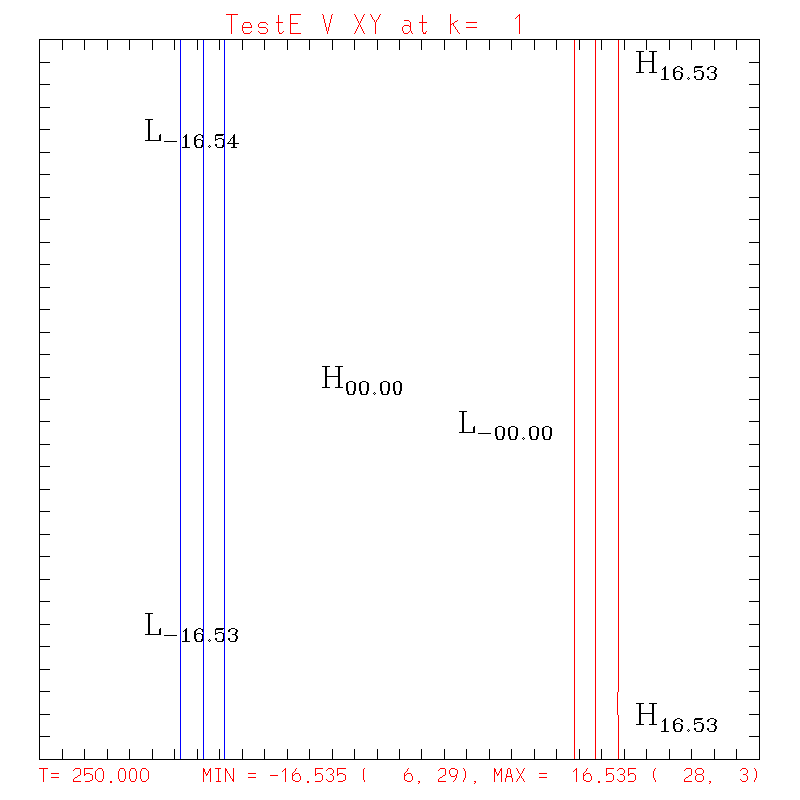
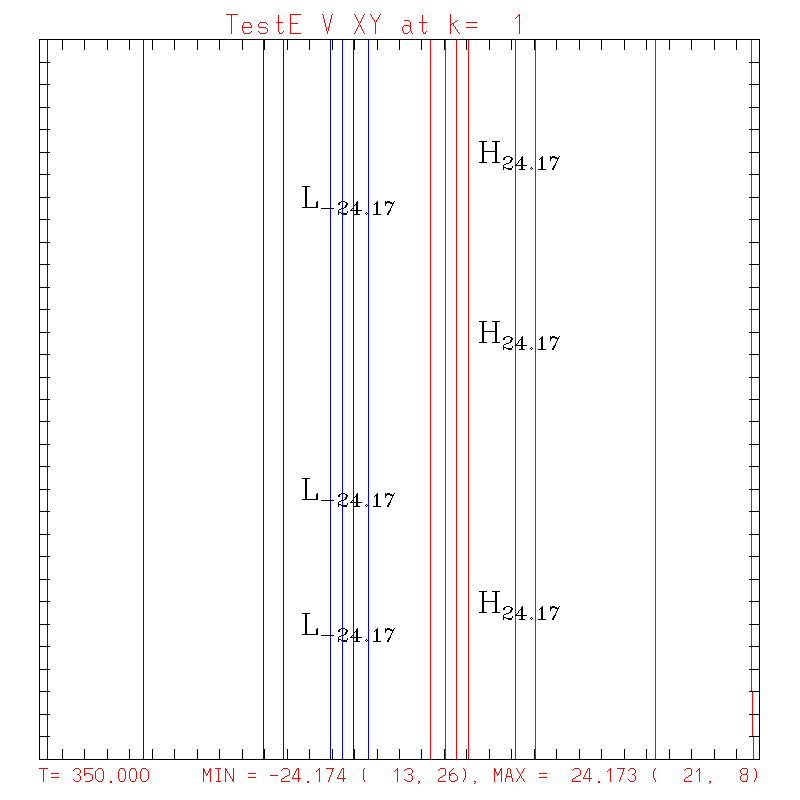
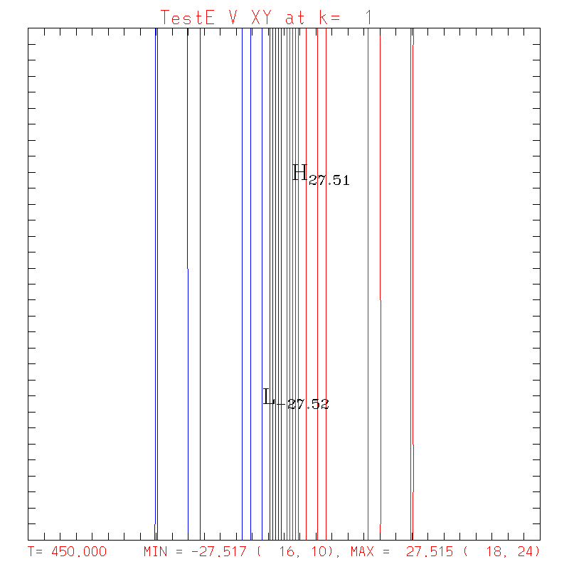
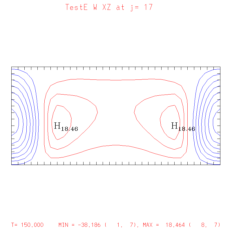
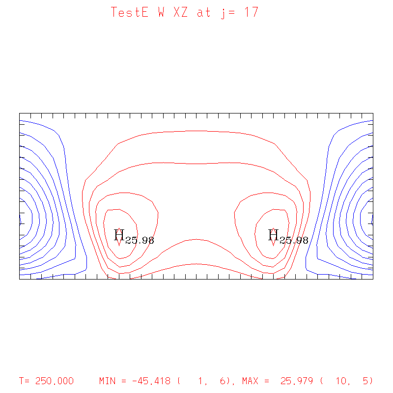
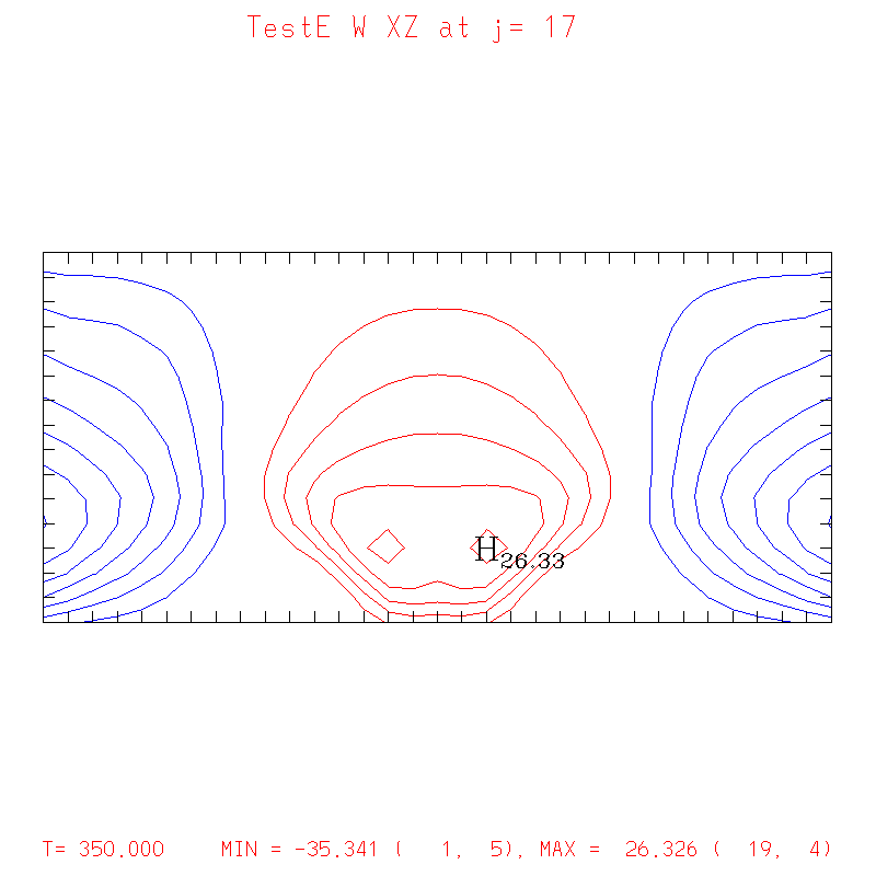
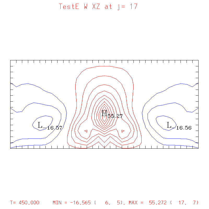
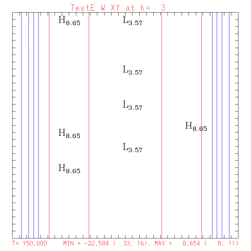
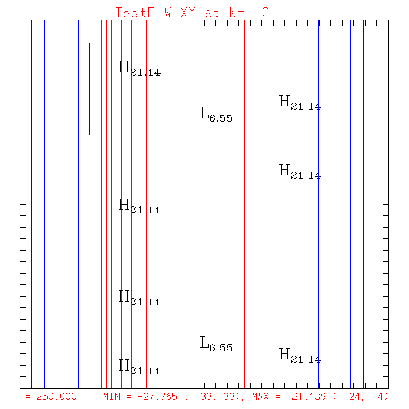
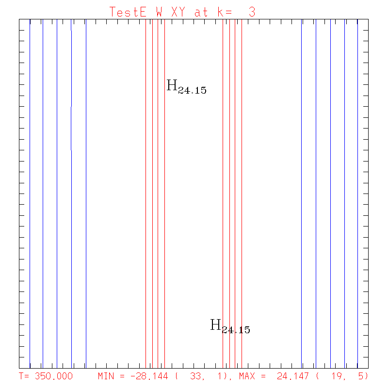
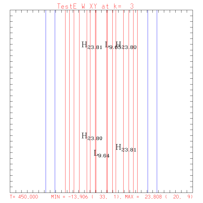
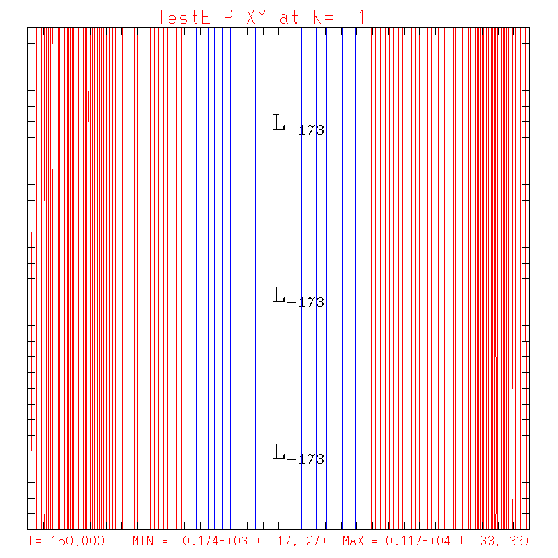
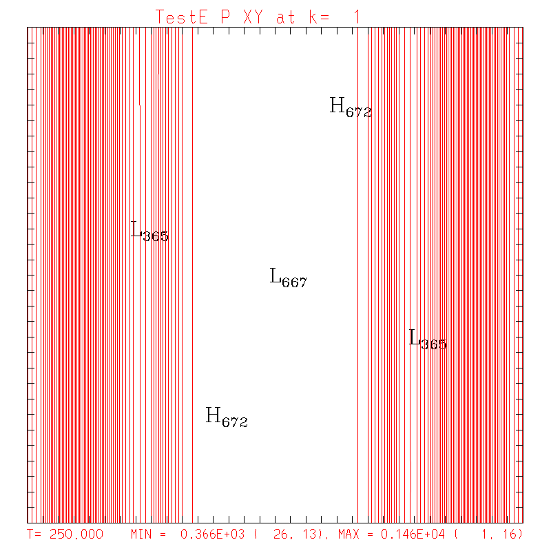
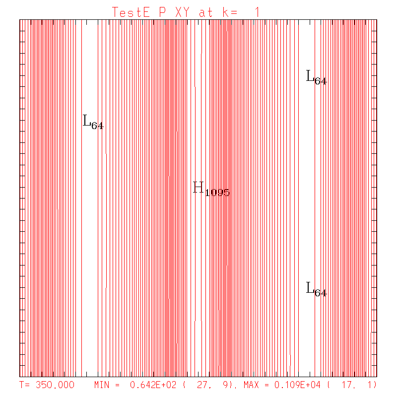
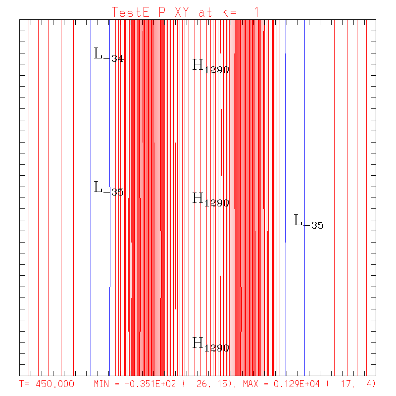
- Contour intervals in plots below are 1˚ (for theta), 5 m/s (for U,V,W), 20 hPa (for P'), and 100 (for vorticity; is actually x10-4 s-1).
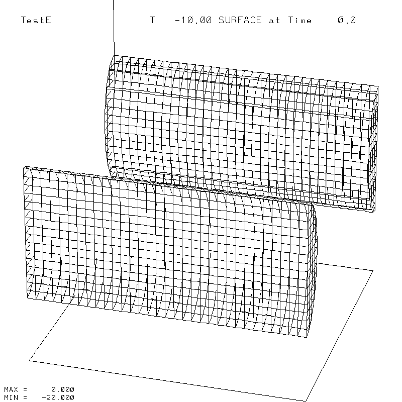
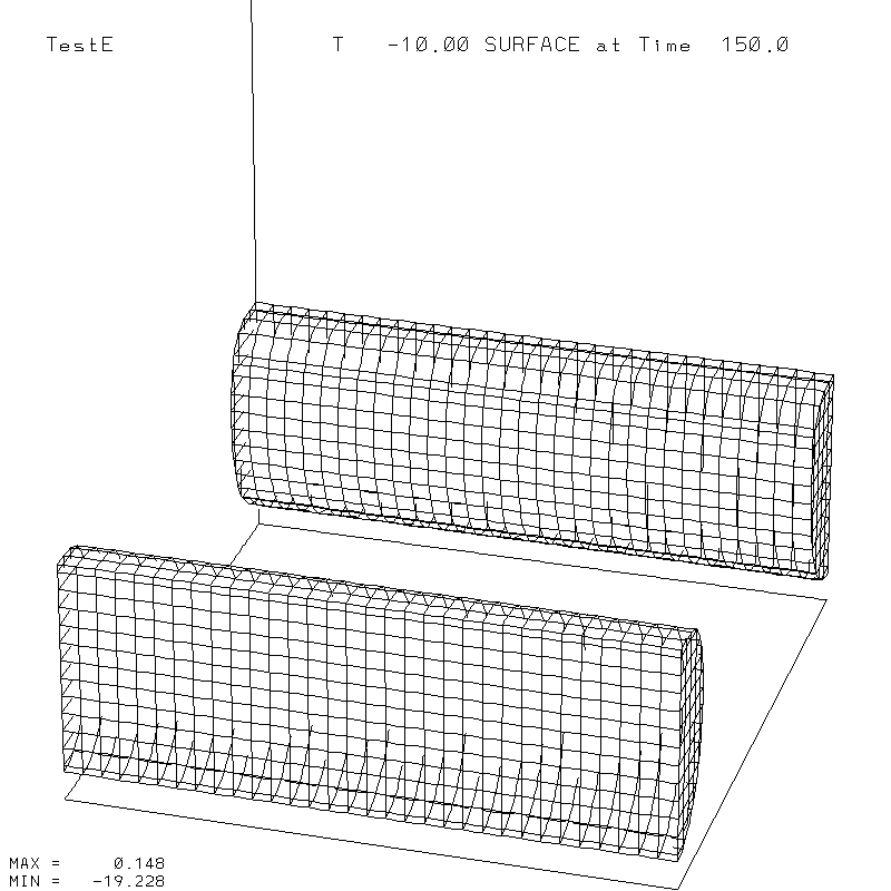
- The 3-D plots use plot3d's default "eye" for viewing (you look towards ~ -X). The isosurface for theta' = -10K, and for vorticity = 100.
- Plot3d will compute vorticity for you (and thus
allow you to plot it), provided you have called putfield with
your U-wind
component named "U" and V-wind component named "V" -- in your call to putfield from your main program.
- As noted elsewhere in the program 6 pages, you can
use plot3d
with a script to generate all the plots you want, at
once.
The script I used for the plots below is available here, named doplot. To use it, copy it to Stampede, tell the system it is an executable script by typing the somewhat arcane Unix command chmod ugo+x doplot, and run it by typing "doplot" as you would any other program. You will see doplot contains the same text you would enter by hand to see the fields. When it finishes you should have a series of ncar metacode files (e.g. Vort_xy.meta). You could then run metagif to convert their contents to GIF.
- It is also possible to put all plots in a single
metacode file; see the Running
Plot3d page for an example of doing so ... you
could then make all the plots into GIFs and combine
them in a zip file to move to your PC with the single
command
~tg457444/502/Tools/metagif filename.meta -all -zip [or, use -tar for a TapeArchive file; most PCs will work with either .tar or .zip]
Or, if you wanted a single file of all images saved as a movie, use
~tg457444/502/Tools/metagif filename.meta -all -gifmovie [or, -qtmovie for Quicktime]
Note either command will leave a pile of .gif files sitting in your directory.
metagif will tell you the file names it is using when making movies.
- I created an
animation of theta by doing the following. I
ran my program, saving output via putfield
every 10 seconds (i.e. every 10 steps in this
case). The RunHistory.dat file was 16039292
bytes. I then ran plot3d as usual, plotting T in
3-D with a -10˚ isosurface, and I used metagif to
convert the resulting metacode file into a series
of GIFs and movies in animated GIF and Quicktime
form. You can see my login
session for the details of what I typed and
the resulting output. The theta animations
are here: GIF,
QT.
Test E |
T=0 | T=150 | T=250 | T=350 | T=450 |
|---|---|---|---|---|---|
| T X-Z |
 |
 |
 |
 |
 |
| T X-Y k=1 |
 |
 |
 |
 |
 |
| T 3-D |
 |
 |
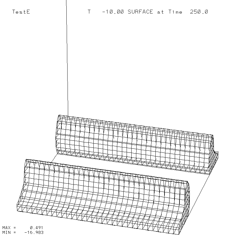 |
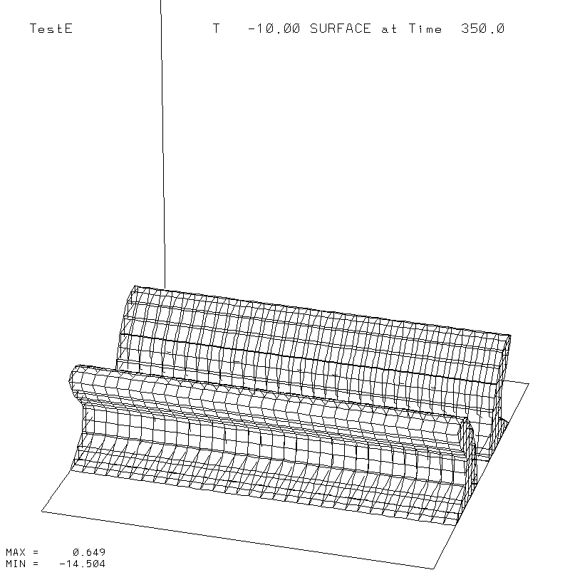 |
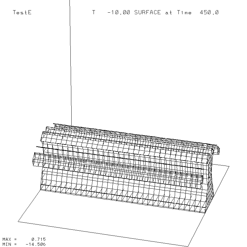 |
| Vorticity X-Z |
 |
 |
 |
 |
 |
| Vorticity X-Y k=1 |
 |
 |
 |
 |
 |
| Vorticity 3-D |
 |
 |
 |
 |
 |
| U X-Z |
 |
 |
 |
 |
 |
| U X-Y k=1 |
 |
 |
 |
 |
 |
| V X-Z |
 |
 |
 |
 |
 |
| V X-Y k=1 |
 |
 |
 |
 |
 |
| W X-Z |
 |
 |
 |
 |
 |
| W X-Y k=3 |
 |
 |
 |
 |
 |
| P X-Z |
 |
 |
 |
 |
 |
| P X-Y k=1 |
 |
 |
 |
 |
 |