Description
- Problem: Linear advection, deformational 2D
flow; cone initial condition
- Method: Lax-Wendroff and 6th-order Crowley, and Takacs
- Domain: 2-D, -0.5 to +0.5 in x and y (for scalar field "s"), same as program #2.
- Due date: 2:00 PM Friday March 1
- Problem handout: PDF
- Corrections to handout:
- initial U, V field formulae should involve 4*pi*x and 4*pi*y, not 3.
- time steps to plot for the official hand-in
problem are 125, 250, 750 steps
Notes on this program
- Questions from last year:
- Do
I need to submit a PDF of the code?
-
Answer: No, a set of code files or tar file is preferred.
- Strange
contour behavior - was found
to be tied to passing an integer (e.g. 0
instead of 0.0) to the
contour routine when it expected a Fortran real or C float value instead. For one student this
resulted in a (very noisy) 0-value contour line to be drawn despite his settings when calling the function. - Asymmetry problems - problem could be in the IC routine or your advection() or advect1d() routines.
- In
IC, make sure your x and y coordinates are
correct when setting up s, u
and v.
Remember - in C - s is set with indices from i1 to i2 and j1 to j2, but u and v indices start at zero! - In
advection(), be careful that you are using
the right u and v values. Again -
especially in C,
you have to simultaneously work in "i1,i1,j2,j2" coordinates (for s) but use u(i-i1,j) (for example).
- In advect1d(), make sure you average the velocity to the s point when computing the Courant number.
- Also
in advect1d(), make sure you use one array
as "input" of s values, and another
as output, so
your expressions look like (within a loop)
s2(i) = s1(i) - ... (Fortran) or s2[i] = s1[i] - ... (in C)
- Array dimensions -- It is recommended to assume 3 ghost points throughout your code but
- if you are a Fortran programmer, still set the nx,ny values only in the global_data module,
- ... so the global_data module defines the arrays as (e.g.) s1(-2:nx+3,-2:ny+3)
- if you are a C programmer, you must
still use the i1,i2,j1,j2 notation.
- So your bc routine will always set
conditions for all 3 ghost points in
every case;
schemes other than 6th-order Crowley just won't use them.
- If you want to be completely
general in your coding (other than in the array
dimensions, that is),
that is fine too - as one student did this way in the past -
for (i=I1; i<=I2; i++) {
for (j=BC_WIDTH; j>0; j--) {
s1[i][j-1] = s1[i][j];
} } /* and so on */
- Variable-dimension arrays: If you want to be completely
general (not required in our class!),
then
read up on allocating float arrays in C within your program, and allocatable arrays in Fortran.
- Initialization:
In function/subroutine ic,
remember to use separate double-loops
for s, u, and v,
and for u to have the X coordinate set to [ the s coordinate minus dx/2.0 ],
and for v to have the Y coordinate set to [ the s coordinate minus dy/2.0 ] ...
and watch out for loop ranges: in Fortran, u will use i=1,nx+1 but v will use i = 1,nx - etc.
- C programmers:
- For the Takacs formula use fabs() instead of abs(); abs is an integer routine, as detailed here.
- Be careful with indices in your Initialization ("ic") routine.
- U,V do not have ghost points. Be careful in computing X,Y.
Program settings, and test case settings/results
Note the differences between the test parameters and your assignment.>> Be sure and change your parameters back to the official problem before running & handing it in!
- Official hand-in problem:
- Domain 351x351, time step 0.002, cone radius 0.100, plot at 125, 250, and 750 steps.
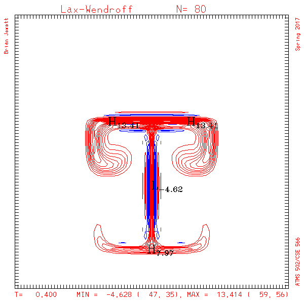
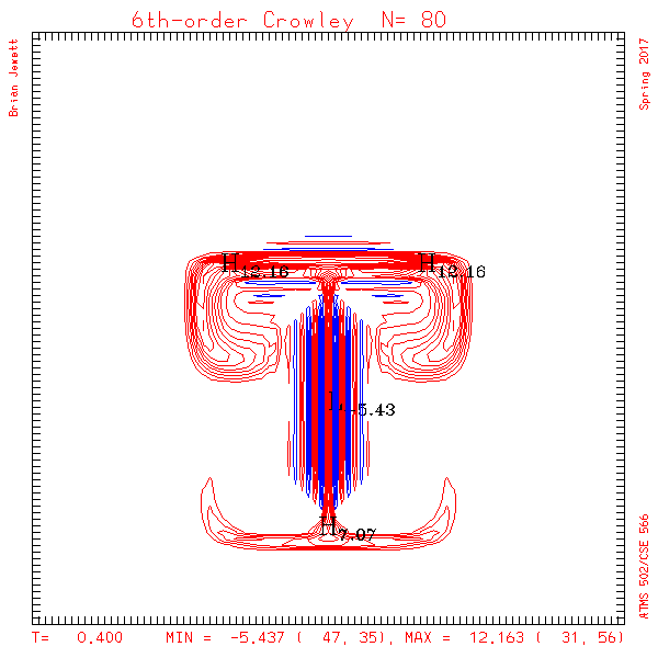
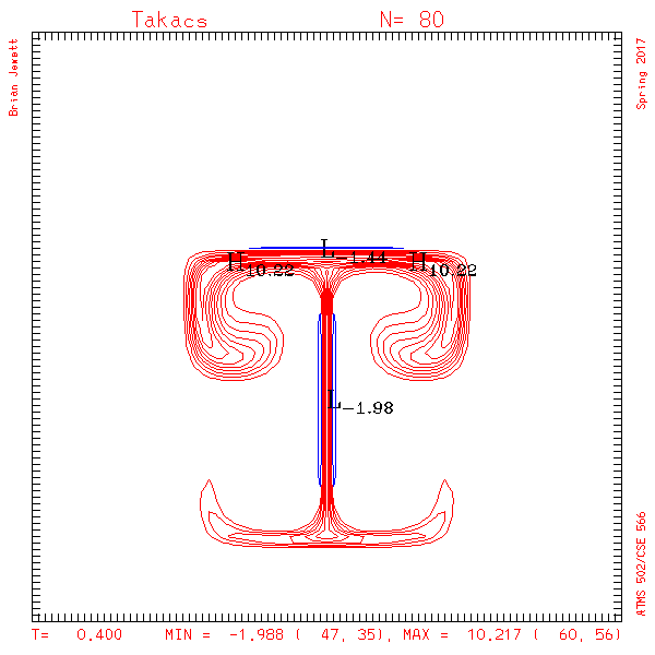
- Test case problem shown below:
- Domain 91x91, time step 0.005,
cone radius 0.200,
plot at 20, 40, 60, 80 steps.
- Cone center is the same for both the test case and official problem: (0.0, -0.05)
- dx=dy calculated same way as in program #2 (dx = 1./real(nx-1), in Fortran)
- Plotting: S contour interval in my plots
is 1.0, U and V contour intervals are 0.1
- A hint: because the velocity field is symmetric about the center X=0, and the initial cone position is at the X-domain center, your solution should maintain near-perfect symmetry about X=0 throughout your simulation. Check this by inspection of your contour plots.
TEST
CASE results are below. I used a contour interval of 1.0
for all of the contour plots.
Click on any image to jump to the web page for
that scheme; click on ">"
to step forward.
| Lax-Wendroff | 6th-order Crowley | Takacs |
|---|---|---|
 |
 |
 |
FAQs, Questions & Answers
- [
Problems with large values near boundaries ]
The problem was in the boundary condition routine, but also in advection.
In (2d) advection, remember to pass nx+1 staggered velocities to advect1d, and also remember to
pass -2:nx+3 values of the scalar s (that is, interior + ghost points) to advect1d.
-
For pgm3, should we put the initial cone center to (0,0) or (0.0, -0.05)?
Can [I] use the knowledge that the number of ghost points is 3 when I organize loops?
I think this is consistent on the web page - finally! Please use (0.0, -0.05). -
Can I "hardcode" the number of ghost zones at the recommended value of 3?
Yes, this is fine.___________________________________ older questions/answers _________________________________________
- I am getting a floating
point exception ...
Presumably this could be a divide-by-zero error but it also could be that your solution is blowing up.
I recommend the following:a) run your code, plotting the output fields every time step. Check the last few plots you were able to get, for any sign of the solution
blowing up (this is more likely to occur near domain boundaries than in the interior)
b) recompile your code, using compile options recommended on page 2 of the computing handout from the first class,
under "to debug your program", and run again to see if any problems show up.
c) print statements - or use of a debugger - are also useful. I print out the min/max values in my code on every time step -
you may find this helpful as well. -
[Fortran] The time shown on the "sfc" plots becomes asterisks ***** on/after T=100 seconds
If so, alter the format statement for writing the time, e.g.
write(tlabel,15) time
15 format('TIME =',f7.4)
Change the format from f7.4 to say f9.4, to handle the larger time values.
I have made this change in my 502/Pgm3 copy of the sfc.f90 routine.
- Should
the Takacs scheme also have a symmetric solution
(about X=0)? Mine is symmetric for other
schemes
Yes it should.
- [beware of checks for 'solution
blowing up']
A holdover from program 1 is checks for "unreasonable" values in your solution. You may be checking to see if smin is below -5, or smax greater than 15. These checks can be commented out or deleted here (plotting smin and smax is not required. I still plot it in my code). The solution - particularly when using Lax-Wendroff - can easily exceed these earlier thresholds. If you want to check for a failing solution, be less restrictive, e.g. "if (smin.lt.-25.0 .or. smax.gt.35.0) then..."
- [more on codes failing with
segmentation faults or behaving different from one run
to another]
Another way in which problems are occurring in Fortran is when updating your 2d array with results from the 1-d array returned by the 1-d advection routine. Your 1-d advection routine only updates the 1d array from 1 to nx, e.g. "s1d_new(1:nx)". If you attempt to copy boundary points - which were not updated by the 1d routine - from this 1d array, this could lead to errors or unpredictable behavior. That is, "s1d_new(nx+1)" was not set by your 1d routine, and so should not be used.
Explanation: this problem is most severe when the 1-d array in question is defined internally in a subroutine. For example, say you pass the dimension "nx" to routine "advection". Inside "advection" you dimension/allocate an array, "real, dimension (-1:nx+2) :: s1d_new", and then proceed to use s1d_new in calls to your 1d advection routine. All well and good, but when you call advection, "s1d_new" is essentially allocated at that time. Its contents, unless you explicitly set them, are undefined. So when s1d_new is returned from advect1d, only the contents from 1 to nx have been set. The other values could contain anything, and trying to access values outside [1,nx] may produce an error - or may not, depending on what was in memory when the program was running. Some computers/compilers will set things to zero for you. You shouldn't count on this. Just because an array has been allocated does not mean its values are defined - unless you define them.
- My code is blowing up
unexpectedly and/or behaving differently when I run it
different times
Compilers can be unforgiving if you move or manipulate data you have not set previously. For example, if you only set values for s1d(1:nx), and try to access s1d(nx+1) -- even if it is dimensioned OK - you may get errors or inconsistent behavior from one run to the next. Here are suggestions that have helped some:
a) compile with "-zero" (this refers to Fortran only).
This initializes all values to zero (integers, real, everything) at the start of the program.
b) set the entire contents of the s1() and s2() arrays to zero before calling your ic() routine.
In Fortran, you can just say "s1=0.0" and "s2=0.0".
- I'm having (code) problems...
* Fortran programmers: Do take advantage of Fortran's additional debugging options.
Compile your code with "-check all -traceback"; it can find common problems with array dimensions or loop bounds.
* In C, use "-g -debug extended -traceback".
* For either: should you not get useful information (particularly, in what routine the program is having e.g. "segmentation fault"),
try running your code within a debugger. One way: usegdb name-of-executable-program
to run it; then type run, then proceed as usual. Type quit to exit the debugger.
- Is the formula for the initial
scalar cone "s" the same as in program 2?
Yes, use the same formula. Note the location of the center, and the cone radius, differ from program 2.
- Won't the physical location of U
and V now extend beyond the [-0.5,+0.5] range of the
domain we are using?
Yes. The range of X and Y between [-0.5,+0.5] applies only to the scalar field S. Since U is staggered 1/2 grid length to the left of S, and since there are nx+1 values of U vs. nx values of S, U(1) will be dx/2 to the left of S(1) and U(nx+1) will be dx/2 to the right of S(nx). Similarly, V (from j=1 to ny+1) will also extend outside the [-0.5,+0.5] physical range.
- Say more about the x, y location
differences for s, u, and v ...
In Program 2, we could get away with using the same x,y locations for the scalar and flow field because U was a function of only Y, and V was only a function of X. This is no longer true. In fact, you should now be using three separate loops for your initial conditions for S, U, and V, because the array sizes and thus do- or for-loop ranges differ between S, U, and V. Relative to the X, Y location of a S point, the location of a U point is (X-dx/2, same Y); the location of a V point is (same X; Y-dy/2).
- The local Courant number
calculations ...
Since U and V are now functions of X and Y, we need to take into account the grid staggering. When computing the local Courant number for a S point for Lax-Wendroff, 6th-order Crowley, or Takacs, average U in the x-direction, and V in the y-direction
[remember, U(i,j) is dx/2 to the left of S(i,j), so the average U at a S point location is 0.5*(u(i,j)+u(i+1,j)) ]
- I noticed that you have plots
of wind vectors in your program 3 example figures.
Would I be able to get access to this routine?
Yes - this is via a NCAR Graphics routine, the simplest of which I am using here (it is not required). I called it as:
call ezvec(uplot,vplot,nx,ny)
where uplot, vplot are my U and V wind components that have been averaged to the S locations.
Documentation on ezvec is available here: http://linux.die.net/man/3/ncl_ezvec
Note: this routine is obsolete - has been replaced by others, documented here: http://ngwww.ucar.edu/supplements/vectors/
- My plots aren't looking like the test
results..
First compare the min/max stats, and note I used a contour interval of 2.0 here, instead of 0.5 from program #2.
I have added a note above to clarify this.