Hands-On, Minds-On Meteorology Description | Programming | Operation Mountains (incl. fixed and large-size versions) Description All three Mountains programs allow the user to follow a parcel of air across a predetermined path of two mountains. The path starts at 0m, progresses upward to 2km, down to 1km, up to 3km, and back to the surface. The only difference between the three is in the original version, you can change the initial temperature and dew point, whereas in the fixed, you can not. The large-size version is like the original -- with adjustable initial temperature and dew point scrollbars. click for whole shot   Objectives The Objective of the Mountains programs is to develop an understanding for what happens to air as it rises and sinks, and how mountains play a role in affecting the properties of the air that passes over it. Programming Theory The path is simply a pair of integer arrays holding x,y data. Clicking start sets off a timer that steps through the path, drawing any pertinent information along the way. 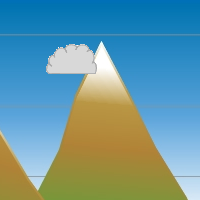Assumptions Range for Initial Temperature Setting: 0°C - 30°C Range for Initial Dew Point Temperature Setting: 0°C - 25°C Initial Temperature and Dew Point Temperature for Fixed version respectively: 25°C and 17°C Dry Lapse Rate for Temperature: 10°C/1000m Dry Lapse Rate for Dew Point Temperature: 2°C/1000m Moist Lapse Rate: 6°C/1000m Cloud formation differs between the fixed version and the others. In the fixed version, we know when the parcel reaches 100%, so we can play a little and allow the cloud to gradually become larger as it ascends above the condensation level. At 1000m, the cloud begins as small, and grows until the parcel begins to sink down the lee side of the first mountain. This cloud quickly shrinks as it descends, so it is visible as the RH < 100%. The parcel stays dry until it returns to 2km, where it again gradually grows to the maximum elevation of the second mountain. The clouds shrinks to nothing over the peak just like the first time. In the adjustable and large-size version, the cloud appears on the screen either in full size or not at all, depending on the relative humidity. In these, as soon as the parcel sinks, the cloud disappears. Equations Nothing other than using the above lapse rates to calculate current temperatures and dew point temperatures. Other Meteogram The red line is the parcel temperature The cyan line is the dew point temperature The yellow vertical line is the marked to show where the parcel currently is on the meteogram. Once Mouse-dragging is enabled (after the first full run at a given temperature setting), the yellow line follows the parcel location to show where it lies on the meteogram. 0°C is the default lower boundary of the meteogram, but it can adjust to accommodate negative numbers by lowering the lower boundary in 10°F increments. Operation Running the Program Click the link for Mountains or Mountains (Large) or Mountains (Fixed). Change the initial parcel temperature and dew point by sliding the appropriate scrollbars. Start and Stop the parcel moving over the mountains by clicking the appropriate button. Enable the Graphing Tool by click the appropriate button. Use the mouse to drag the parcel to any point along the path only after the path is run once. Press reset to start a new parcel experiment (the only way to change initial temp / dew point in adjustable version) Extra Knowledge The students can drag the parcel along its track, only once the track has been run through completely on its own. Department of Atmospheric Sciences University of Illinois at Urbana Champaign Created by Dan Bramer: Last Modified 07/27/2004 send questions/comments to bramer@atmos.uiuc.edu